3 Excel tricks that few people know

My goal is to uncover those secrets hidden in Excel that can radically transform the efficiency and effectiveness with which we work in our spreadsheets.

1. Using pivot tables to summarize data

The Dynamic tables They are powerful tools for summarizing, analyzing, exploring, and presenting data. Although many users are aware of its existence, few take advantage of its ability to quickly transform large volumes of data into understandable reports.

Practical example: Sales analysis by product and region

Context: Imagine that you work with a sales database that includes detailed information about products sold, the date of sale, the region of sale, and the amount of each sale. Our goal is to summarize this information to better understand which products are selling the most in each region.

Step 1: Prepare the data

Make sure your data is organized in a clear table, with each column representing a variable (Product, Date, Region, Sales Amount), and each row representing a sale.

Step 2: Create the PivotTable

• Select any cell within your data set.
• Go to tab Insert and choose Dynamic table.
• Excel will ask you if you want to create the pivot table in an existing sheet or a new one. Choose “New sheet» to keep your analysis clean and organized.
• Click Accept.

Step 3: Configure the PivotTable

Once you are in the new sheet with the pivot table area:

• Drag the “Region” field to the area of Rows. This will create a list of all the regions in your data set.
• Drag the “Product” field to the Columns. This will disperse the products across the top of the table.
• Drag the “Sales Amount” field to the sales area. Values. This will automatically add sales by product and region.

Step 4: Analyze the data

Now, you have a dynamic table that summarizes the total sales amount of each product by region. You can easily identify which products are the best sellers in each region and where you might need to adjust your sales or marketing strategies.

Step 5: Customize and Deepen

Pivot tables are highly customizable. Can:

• Filter data to view only certain regions or products.
• Order the data to see the best-selling products at the top.
• Add calculation fields to analyze profit margins.
• Wear data slicers for quick and visual filtering.

2. Custom keyboard shortcuts

Excel allows you to create custom keyboard shortcuts through macros, a feature that can save a lot of time. Automating repetitive tasks using macros and assigning them a specific keyboard shortcut is a trick that significantly increases productivity.

I’m going to walk you through how you can create a custom keyboard shortcut for a common task: inserting the current date and time into a selected cell. This feature is very useful when you are documenting records or updates in your spreadsheets.

Practical example: Create a shortcut to insert current Date and Time

Step 1: Open VBA Editor

• Press Alt + F11 to open the Visual Basic for Applications (VBA) Editor in Excel.

Step 2: Insert a New Module

• In the menu Insert From the VBA Editor, select Module. This will create a new module.

Step 3: Write the Code for the Macro

• In the module you just created, write the following VBA code:
• Sub InsertDateTime()
  ActiveCell.Value = Now
  ActiveCell.NumberFormat = “dd/mm/yyyy hh:mm:ss”
  End Sub

This code assigns the active cell (the selected cell) the current date and time (Now) and then applies a specific date and time format.

Step 4: Save the Macro

• Save the book Excel with the format of Excel macro-enabled workbook (.xlsm) to make sure the macro is saved with your file.

Step 5: Assign a Keyboard Shortcut to the Macro

To assign a custom keyboard shortcut to your macro:

• Go back to Excel and go to the tab View.
• Click MacrosChoose View Macros.
• Select the macro InsertarFechaHora that you just created.
• Click Options…
• In the countryside Shortcut key, enter a letter that will be the keyboard shortcut. For example, enter f will assign Ctrl + f as the shortcut for this macro. Choose a key combination that doesn’t interfere with Excel’s default keyboard shortcuts.
• Click Accept and close the dialog box.

Step 6: Use the Keyboard Shortcut

• Now, simply select any cell on your sheet. Excelpress Ctrl + f (or whatever key combination you chose), and the current date and time will be automatically inserted into the cell.

This method not only saves you time, but also allows you to customize Excel to adapt it to your specific needs.

3. VLOOKUP function with fuzzy match

The function VLOOKUP is known, but its ability to perform fuzzy-match searches is often underestimated. This functionality can be crucial when working with data that is not perfectly uniform.

Here I will show you how to use VLOOKUP with a fuzzy match, which is ideal when the values ​​you are looking for are not exact or when you are working with ranges of values ​​rather than single values.

Practical Example: Determine the discount based on purchase volume

Imagine that you have a list of discounts based on purchase volume for your customers. For each purchase volume range, there is a corresponding discount percentage. You want to automate the process to determine the applicable discount based on a customer’s purchase volume.

Step 1: Create the Discount Table

First, you need a table that specifies volume ranges and corresponding discounts. Let’s say your table looks like this:

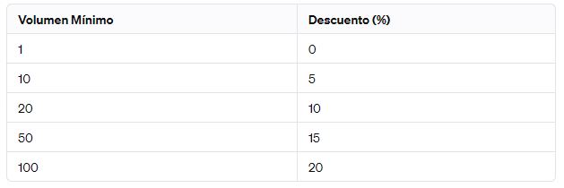
This table indicates, for example, that purchases of 10 or more (up to 19) receive a 5% discount, and purchases of 20 or more (up to 49) receive a 10% discount, etc.

Step 2: Use VLOOKUP to Find the Discount

Let’s say you want to find the discount for a purchase of 25 units. The function VLOOKUP can be set to search for a fuzzy match like this:

• =VLOOKUP(A2, A:B, 2, TRUE)

In this case, A2 contains the purchase volume (25 units), A:B is the range where the discount table is located, 2 indicates that we want to return the value of the second column (Discount %), and VERDADERO specifies that we are looking for a fuzzy match.

Step 3: Understand the Result

Excel will look in the Minimum Volume column for the value closest to 25 without going over. It finds that 20 is the closest value that does not exceed 25, so it returns the discount associated with 20, which is 10%.

This approach is particularly useful for lookup tables where exact values ​​may not be present, and you need to determine which “category” or “range” a given value belongs to.

Each of these tricks, while they may seem simple at first glance, has the potential to significantly change how we interact with Excel, taking our data analysis and presentation skills to a new level. At Mediaboooster, we always seek to highlight these hidden gems of technology, ensuring that our audience not only stays informed, but also a step ahead in mastering such essential tools as Excel. If we see that there is success with these tricks, we will continue with more of them in future articles.